- Hypothesis Testing with Laplacian Noise
A random variable N is said to be Laplacian distributed if its probability density function is given by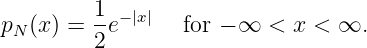
Consider the following decision problem involving the observed random variable Z:
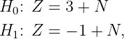
where the two hypotheses are equally likely.
- Provide expressions for the probability density function for Z for each of the two hypotheses.
- Show that the maximum likelihood decision rule can be
simplified to

Determine the value of the optimum threshold γ.
- Compute the probability of error for this decision rule.
For the remainder of the problem, consider a two-dimensional random vector
 =
= 
N1 N2  with independent Laplacian distributed components, i.e.,

with
 =
= 
x1 x2  .
.
Consider the following decision problem involving the observed random vector
 =
= 
Z1 Z2  :
:
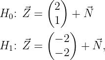
where again the two hypotheses are equally likely.
- Provide expressions for the probability density function for
 for each of the two hypotheses.
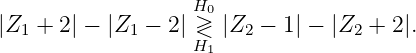
- Show that the maximum likelihood decision rule can be
simplified to
- The absolute values in the decision rule induce three distinct
intervals for Z1 (Z1 < -2, -2 ≤ Z1 ≤ 2, and Z1 > 2) and
three intervals for Z2 (Z2 < -2, -2 ≤ Z2 ≤ 1, and Z2 > 1).
Consider all nine regions formed by combinations of these intervals (e.g., the region with Z1 < -2 and Z2 < -2) and simplify the decision rule for each of these combinations.
- Draw a two-dimensional signal-space diagram with axes Z1
and Z2. Mark the locations of E[
 |Hi] for the two hypotheses.
Then, draw the decision boundary formed by the optimal
decision rule using the results from part (f).
|Hi] for the two hypotheses.
Then, draw the decision boundary formed by the optimal
decision rule using the results from part (f).
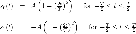
- Binary Signal Sets
The following signal set is employed to transmit equally likely signals over an additive white Gaussian noise channel with spectral height .
.
- Sketch and accurately label the block diagram of a receiver that minimizes the probability of error.
- Compute the energy of each of the two signals.
- Compute the probability of error for your receiver from part (a).
- Consider now the following receiver:
Find the conditional distribution of the random variable
R at the output of the integrator for each of the two signalss 0 (t ) ands 1 (t ). - Compute the probability of error achieved by the suboptimum receiver.
- Compare the probability of error for the suboptimum receiver to
that of the optimum receiver. Express your answer in the form: “to
achieve the same probability of error as the optimum receiver, the
suboptimum system requires
a times more energy.” Determine the factora . - Assume now that the received signal is corrupted by an
interfering signal
x (t ) = , for
, for - 
≤ t ≤  so that the
received signal under the
so that the
received signal under the i -th hypotesis (i = 0, 1) is given by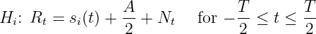
Compute the probability of error by the optimum receiver in the presence of the interfering signal.
- Explain your result in part (g).